Tutorials
This page provides useful tutorials for running PyPGx. Throughout the page, it’s assumed that you have installed the latest version of PyPGx and also downloaded the appropriate resource bundle (i.e. matching version). For more details, please see Installation and Resource bundle.
GeT-RM WGS tutorial
In this tutorial I’ll walk you through PyPGx’s genotype analysis using whole genome sequencing (WGS) data. By the end of this tutorial, you will have learned how to perform genotype analysis for genes with or without structural variation (SV), accordingly. I will also show how PyPGx can handle genomic data from two different Genome Reference Consortium Human (GRCh) builds: GRCh37 (hg19) and GRCh38 (hg38).
Before beginning this tutorial, create a new directory and change to that directory:
$ mkdir getrm-wgs-tutorial
$ cd getrm-wgs-tutorial
The Centers for Disease Control and Prevention–based Genetic Testing Reference Materials Coordination Program (GeT-RM) has established genomic DNA reference materials to help the genetic testing community obtain characterized reference materials. In particular, GeT-RM has made WGS data for 70 of reference samples publicly available for download and use from the European Nucleotide Archive. We will be using this WGS dataset throughout the tutorial.
Obtaining input files
Because downloading the entire WGS dataset is probably not feasible for most users due to large file size (i.e. a 30x WGS sample ≈ 90 GB), I have prepared input files ranging from 2 KB to 25.5 MB, for both GRCh37 and GRCh38. You can easily download these with:
$ wget https://raw.githubusercontent.com/sbslee/pypgx-data/main/getrm-wgs-tutorial/grch37-variants.vcf.gz
$ wget https://raw.githubusercontent.com/sbslee/pypgx-data/main/getrm-wgs-tutorial/grch37-variants.vcf.gz.tbi
$ wget https://raw.githubusercontent.com/sbslee/pypgx-data/main/getrm-wgs-tutorial/grch37-depth-of-coverage.zip
$ wget https://raw.githubusercontent.com/sbslee/pypgx-data/main/getrm-wgs-tutorial/grch37-control-statistics-VDR.zip
$ wget https://raw.githubusercontent.com/sbslee/pypgx-data/main/getrm-wgs-tutorial/grch38-variants.vcf.gz
$ wget https://raw.githubusercontent.com/sbslee/pypgx-data/main/getrm-wgs-tutorial/grch38-variants.vcf.gz.tbi
$ wget https://raw.githubusercontent.com/sbslee/pypgx-data/main/getrm-wgs-tutorial/grch38-depth-of-coverage.zip
$ wget https://raw.githubusercontent.com/sbslee/pypgx-data/main/getrm-wgs-tutorial/grch38-control-statistics-VDR.zip
Let’s take a look at the metadata for some of these files. If you’re not
familiar with what metadata is, please visit Archive file, semantic type,
and metadata. The first one we’ll
look at is an archive file with the semantic type
CovFrame[DepthOfCoverage]:
$ pypgx print-metadata grch37-depth-of-coverage.zip
Assembly=GRCh37
SemanticType=CovFrame[DepthOfCoverage]
Platform=WGS
We can see that above archive was created using WGS data aligned to GRCh37. It has following data structure:
$ pypgx print-data grch37-depth-of-coverage.zip | head
Chromosome  Position        NA18519_PyPGx   HG01190_PyPGx   NA12006_PyPGx   NA18484_PyPGx   NA07055_PyPGx   NA18980_PyPGx   NA19213_PyPGx   NA12813_PyPGx   NA19003_PyPGx   NA10831_PyPGx   NA18524_PyPGx   NA10851_PyPGx   NA18966_PyPGx   HG00589_PyPGx   NA18855_PyPGx   NA18544_PyPGx   NA18518_PyPGx   NA18973_PyPGx   NA19143_PyPGx   NA18992_PyPGx   NA12873_PyPGx   NA19207_PyPGx   NA18942_PyPGx   NA19178_PyPGx   NA19789_PyPGx   NA19122_PyPGx   NA19174_PyPGx   NA18868_PyPGx   HG00436_PyPGx   HG00276_PyPGx   NA19239_PyPGx   NA19109_PyPGx   NA20509_PyPGx   NA10854_PyPGx   NA19226_PyPGx   NA10847_PyPGx   NA18552_PyPGx   NA18526_PyPGx   NA07029_PyPGx   NA06991_PyPGx   NA11832_PyPGx   NA21781_PyPGx   NA12145_PyPGx   NA19007_PyPGx   NA18861_PyPGx   NA12156_PyPGx   NA18952_PyPGx   NA18565_PyPGx   NA19920_PyPGx   NA12003_PyPGx   NA20296_PyPGx   NA07019_PyPGx   NA07056_PyPGx   NA11993_PyPGx   NA19147_PyPGx   NA19819_PyPGx   NA07000_PyPGx   NA18540_PyPGx   NA19095_PyPGx   NA18509_PyPGx   NA19917_PyPGx   NA18617_PyPGx   NA07357_PyPGx   NA19176_PyPGx   NA18959_PyPGx   NA07348_PyPGx   NA18564_PyPGx   NA19908_PyPGx   NA11839_PyPGx   NA12717_PyPGx
chr1        110227417       17      0       9       12      12      13      10      0       0       0       0       1       14      10      4       26      7       6       0       0       4       19      8       6       0       15      0       17      20      0       0       15      10      11      0       7       18      0       0       0       0       22      11      0       6       0       0       0       24      17      17      12      19      0       14      0       0       13      15      8       0       24      0       10
chr1        110227418       17      0       9       12      12      13      10      0       0       0       0       1       14      10      4       26      8       8       0       0       4       19      9       6       0       15      0       18      20      0       0       16      10      11      0       8       18      0       0       0       0       22      11      0       6       0       0       0       24      17      17      12      20      0       14      0       0       13      15      8       0       24      0       10
chr1        110227419       17      0       10      12      12      13      10      0       0       0       0       1       14      10      4       27      8       8       0       0       5       19      9       6       0       16      0       18      20      0       0       16      11      11      0       8       18      0       0       0       0       22      12      0       6       0       0       0       24      17      17      12      20      0       14      0       0       14      15      8       0       24      0       10
chr1        110227420       17      0       10      13      13      12      10      0       0       0       0       1       14      10      3       27      8       8       0       0       5       18      9       6       0       15      0       18      19      0       0       16      11      11      0       8       16      0       0       0       0       22      12      0       6       0       0       0       24      19      17      11      19      0       13      0       0       14      15      8       0       23      0       10
chr1        110227421       17      0       10      13      13      12      10      0       0       0       0       1       13      10      3       27      8       8       0       0       5       18      8       7       0       15      0       19      19      0       0       16      11      11      0       8       15      0       0       0       0       22      12      0       6       0       0       0       25      20      17      11      19      0       13      0       0       15      15      8       0       23      0       10
chr1        110227422       18      0       10      13      13      12      10      0       0       0       0       1       13      10      3       27      8       8       0       0       5       18      9       7       0       15      0       19      19      0       0       17      11      11      0       8       15      0       0       0       0       21      12      0       6       0       0       0       25      20      18      11      19      0       13      0       0       16      15      9       0       23      0       10
chr1        110227423       18      0       10      13      13      12      10      0       0       0       0       1       13      10      3       25      8       8       0       0       5       18      9       7       0       15      0       19      18      0       0       17      11      11      0       9       15      0       0       0       0       21      13      0       6       0       0       0       25      20      18      11      19      0       13      0       0       17      15      9       0       23      0       10
chr1        110227424       18      0       10      13      13      12      10      0       0       0       0       1       13      10      3       25      8       8       0       0       5       18      9       7       0       15      0       19      18      0       0       17      11      11      0       9       15      0       0       0       0       21      13      0       6       0       0       0       26      20      18      11      19      0       14      0       0       16      15      9       0       23      0       10
chr1        110227425       19      0       11      13      13      12      10      0       0       0       0       1       13      10      3       25      8       8       0       0       5       18      9       8       0       15      0       20      18      0       0       17      11      11      0       9       15      0       0       0       0       21      13      0       6       0       0       0       26      20      18      13      19      0       15      0       0       16      15      9       0       23      0       10
The second one is an archive file with the semantic type
SampleTable[Statistics]:
$ pypgx print-metadata grch38-control-statistics-VDR.zip
Control=VDR
Assembly=GRCh38
SemanticType=SampleTable[Statistics]
Platform=WGS
Note that this archive was created using WGS data aligned to GRCh38 and the VDR gene as control locus, and has following data structure:
$ pypgx print-data grch38-control-statistics-VDR.zip | head
    count   mean    std     min     25%     50%     75%     max
NA19213_PyPGx       69459.0 40.464317079140216      7.416070659882781       5.0     35.0    40.0    45.0    67.0
HG00436_PyPGx       69459.0 39.05070617198635       7.041075412533929       3.0     34.0    39.0    44.0    66.0
NA12006_PyPGx       69459.0 44.49780446018514       7.565078889270334       6.0     39.0    44.0    50.0    73.0
NA12156_PyPGx       69459.0 39.53788565916584       7.463158820634827       3.0     34.0    39.0    44.0    66.0
NA12813_PyPGx       69459.0 37.33543529276264       6.920597209929764       7.0     33.0    37.0    42.0    67.0
NA19207_PyPGx       69459.0 40.59959112570005       7.042408883522744       4.0     36.0    41.0    45.0    63.0
NA07029_PyPGx       69459.0 38.69389136037086       7.075488283784741       2.0     34.0    39.0    44.0    67.0
NA18980_PyPGx       69459.0 34.79616752328712       6.685174389736681       1.0     30.0    35.0    39.0    59.0
NA18973_PyPGx       69459.0 36.43840251083373       7.0885860461926296      3.0     32.0    37.0    41.0    66.0
Finally, we’ll look at the input VCF. Note that it’s not an archive file per se, but we can still peek at its data:
$ zcat grch37-variants.vcf.gz | grep "#CHROM" -A 5
#CHROM      POS     ID      REF     ALT     QUAL    FILTER  INFO    FORMAT  NA18519_PyPGx   HG01190_PyPGx   NA12006_PyPGx   NA18484_PyPGx   NA07055_PyPGx   NA18980_PyPGx   NA19213_PyPGx   NA12813_PyPGx   NA19003_PyPGx   NA10831_PyPGx   NA18524_PyPGx   NA10851_PyPGx   NA18966_PyPGx   HG00589_PyPGx   NA18855_PyPGx   NA18544_PyPGx   NA18518_PyPGx   NA18973_PyPGx   NA19143_PyPGx   NA18992_PyPGx   NA12873_PyPGx   NA19207_PyPGx   NA18942_PyPGx   NA19178_PyPGx   NA19789_PyPGx   NA19122_PyPGx   NA19174_PyPGx   NA18868_PyPGx   HG00436_PyPGx   HG00276_PyPGx   NA19239_PyPGx   NA19109_PyPGx   NA20509_PyPGx   NA10854_PyPGx   NA19226_PyPGx   NA10847_PyPGx   NA18552_PyPGx   NA18526_PyPGx   NA07029_PyPGx   NA06991_PyPGx   NA11832_PyPGx   NA21781_PyPGx   NA12145_PyPGx   NA19007_PyPGx   NA18861_PyPGx   NA12156_PyPGx   NA18952_PyPGx   NA18565_PyPGx   NA19920_PyPGx   NA12003_PyPGx   NA20296_PyPGx   NA07019_PyPGx   NA07056_PyPGx   NA11993_PyPGx   NA19147_PyPGx   NA19819_PyPGx   NA07000_PyPGx   NA18540_PyPGx   NA19095_PyPGx   NA18509_PyPGx   NA19917_PyPGx   NA18617_PyPGx   NA07357_PyPGx   NA19176_PyPGx   NA18959_PyPGx   NA07348_PyPGx   NA18564_PyPGx   NA19908_PyPGx   NA11839_PyPGx   NA12717_PyPGx
chr1        47261780        .       T       C       235.707 PASS    DP=1519;VDB=0.326231;SGB=-40.8249;RPBZ=0.398415;MQBZ=-15.2308;MQSBZ=0.889911;BQBZ=-10.8447;SCBZ=0.105486;FS=0;MQ0F=0;AC=120;AN=140;DP4=205,13,1153,122;MQ=49    GT:PL:AD        0/0:0,57,255:19,0       0/1:204,0,172:10,11     1/1:240,45,0:0,15       0/1:147,0,165:11,10     1/1:246,54,0:0,18       1/1:255,66,0:0,22       0/1:134,0,182:15,9      1/1:255,87,0:0,29       1/1:231,54,0:0,18       1/1:224,57,0:0,19       1/1:248,36,0:0,12       0/1:120,0,176:9,7       1/1:255,54,0:0,18       1/1:198,75,0:0,25       0/1:168,0,127:7,12      1/1:255,57,0:0,19       0/1:105,0,183:9,5       1/1:223,51,0:0,17       1/1:255,63,0:0,21       1/1:255,80,0:1,31       1/1:189,60,0:0,20       0/1:148,0,214:10,12     1/1:191,45,0:0,15       0/1:98,0,175:15,6       1/1:255,69,0:0,23       0/1:158,0,100:7,16      0/1:161,0,114:5,12      0/1:255,0,138:9,14      1/1:247,81,0:0,27       1/1:227,57,0:0,19       1/1:255,63,0:0,21       1/1:255,69,0:0,23       1/1:255,75,0:0,25       1/1:255,84,0:0,28       0/1:202,0,190:14,15     1/1:224,69,0:0,23       1/1:255,66,0:0,22       1/1:255,63,0:0,21       1/1:255,39,0:0,13       1/1:255,51,0:0,17       1/1:255,72,0:0,24       1/1:231,63,0:0,21       1/1:255,78,0:0,26       1/1:255,75,0:0,25       0/1:145,0,227:16,10     1/1:200,72,0:0,24       1/1:205,72,0:0,24       1/1:207,66,0:0,22       0/1:109,0,172:12,8      0/1:174,0,135:9,14      1/1:255,66,0:0,22       1/1:255,45,0:0,15       1/1:249,54,0:0,18       1/1:255,54,0:0,18       1/1:230,72,0:0,24       1/1:247,63,0:0,21       1/1:211,81,0:0,27       1/1:255,54,0:0,18       0/1:167,0,193:13,13     1/1:255,72,0:0,24       0/1:76,0,159:11,4       1/1:236,66,0:0,22       1/1:255,78,0:0,26       1/1:218,45,0:0,15       1/1:255,60,0:0,20       1/1:255,66,0:0,22       1/1:202,78,0:0,26       1/1:255,81,0:0,27       0/1:181,0,176:16,11     1/1:231,33,0:0,11
chr1        47261821        .       G       A       174.846 PASS    DP=1722;VDB=0.413935;SGB=-18.2343;RPBZ=0.238211;MQBZ=-1.89867;MQSBZ=6.49061;BQBZ=1.3413;SCBZ=0.173613;FS=0;MQ0F=0;AC=1;AN=140;DP4=1407,277,14,2;MQ=52   GT:PL:AD        0/0:0,81,255:27,0       0/0:0,84,255:28,0       0/0:0,60,255:20,0       0/0:0,90,239:30,0       0/0:0,60,221:20,0       0/0:0,84,255:28,0       0/0:0,84,241:28,0       0/0:0,81,255:27,0       0/0:0,63,190:21,0       0/1:200,0,127:11,110/0:0,63,255:21,0    0/0:0,75,255:25,0       0/0:0,63,255:21,0       0/0:0,63,215:21,0       0/0:0,69,216:23,0       0/0:0,75,255:25,0       0/0:0,54,244:18,0       0/0:0,57,212:19,0       0/0:0,90,255:30,0       0/0:0,96,255:32,0       0/0:0,72,241:24,0       0/0:0,72,223:24,0       0/0:0,54,191:18,0       0/0:0,75,223:25,0       0/0:0,75,255:25,0       0/0:0,90,222:30,0       0/0:0,54,180:18,0       0/0:0,99,255:33,0       0/0:0,93,255:31,0       0/0:0,66,212:22,0       0/0:0,72,255:24,0       0/0:0,75,243:25,0       0/0:0,72,255:24,0       0/0:0,69,255:27,1       0/0:0,102,250:34,0      0/0:0,81,186:27,0       0/0:0,66,255:22,0       0/0:0,72,255:24,0       0/0:0,50,236:21,1       0/0:0,60,255:20,0       0/0:0,75,255:25,0       0/0:0,54,182:18,0       0/0:0,75,255:25,0       0/0:0,78,255:26,0       0/0:0,81,233:27,0       0/0:0,78,153:26,0       0/0:0,75,180:25,0       0/0:0,60,174:20,0       0/0:0,51,189:17,0       0/0:0,84,234:28,0       0/0:0,63,255:21,0       0/0:0,48,210:16,0       0/0:0,63,231:21,0       0/0:0,69,255:23,0       0/0:0,81,252:27,0       0/0:0,69,178:23,0       0/0:0,69,221:23,0       0/0:0,57,255:19,0       0/0:0,75,217:25,0       0/0:0,93,255:31,0       0/0:0,54,231:18,0       0/0:0,96,211:32,0       0/0:0,93,255:31,0       0/0:0,54,211:18,0       0/0:0,66,243:22,0       0/0:0,72,222:24,0       0/0:0,90,236:30,0       0/0:0,78,242:26,0       0/0:0,87,255:29,0       0/0:0,45,255:15,0
chr1        47261822        .       A       T       232.856 PASS    DP=1729;VDB=0.568499;SGB=-11.6626;RPBZ=-0.581723;MQBZ=-14.8734;MQSBZ=6.53808;BQBZ=1.09344;SCBZ=1.03879;FS=0;MQ0F=0;AC=88;AN=140;DP4=544,110,864,174;MQ=52       GT:PL:AD        0/0:0,81,255:27,0       0/1:255,0,226:12,17     1/1:255,60,0:0,20       0/0:0,87,255:29,0       0/0:0,63,255:21,0       0/1:152,0,255:15,11     0/1:182,0,223:17,11     1/1:255,81,0:0,27       0/1:128,0,189:13,8      1/1:255,69,0:0,23       1/1:255,66,0:0,22       0/1:246,0,193:11,14     1/1:255,60,0:0,20       1/1:255,60,0:0,20       0/0:0,66,255:22,0       1/1:255,75,0:0,25       0/0:0,54,255:18,0       1/1:255,54,0:0,18       0/1:209,0,255:19,10     0/1:255,0,255:16,161/1:255,72,0:0,24    0/1:145,0,248:15,10     0/1:113,0,170:9,6       0/1:153,0,206:16,8      1/1:255,69,0:0,23       0/0:0,87,255:29,0       0/1:149,0,187:9,10      0/1:255,0,171:12,20     0/1:176,0,255:16,13     0/1:218,0,145:11,130/1:221,0,218:14,10  0/1:237,0,184:11,15     1/1:255,72,0:0,24       1/1:255,84,0:0,28       0/1:254,0,194:16,181/1:255,75,0:0,25    1/1:255,60,0:0,20       1/1:255,69,0:0,23       0/0:0,69,255:23,0       0/0:0,60,255:20,0       1/1:255,72,0:0,24       1/1:236,54,0:0,18       1/1:255,75,0:0,25       0/1:155,0,255:18,10     0/0:0,81,255:27,0       1/1:212,75,0:0,25       0/1:196,0,133:10,15     0/1:171,0,155:9,11      0/1:105,0,188:10,7      0/1:182,0,219:14,131/1:255,63,0:0,21    1/1:255,48,0:0,16       1/1:255,63,0:0,21       1/1:255,72,0:0,24       1/1:255,78,0:0,26       1/1:232,63,0:0,21       0/0:0,66,255:22,0       0/1:150,0,215:10,7      0/1:180,0,178:13,12     0/1:243,0,190:12,180/1:106,0,222:11,6   0/1:212,0,193:13,19     1/1:255,87,0:0,29       1/1:255,57,0:0,19       0/1:203,0,189:9,13      1/1:255,69,0:0,23       0/1:233,0,146:9,20      0/0:0,81,255:27,0       0/1:180,0,249:19,9      1/1:255,45,0:0,15
chr1        47261869        .       C       T       235.707 PASS    DP=1863;VDB=0.677143;SGB=5.02317;RPBZ=-2.55997;MQBZ=-8.87433;MQSBZ=3.1481;BQBZ=26.6865;SCBZ=0.647961;FS=0;MQ0F=0;AC=88;AN=140;DP4=522,174,834,311;MQ=56 GT:PL:AD        0/0:0,84,255:28,0       0/1:255,0,194:12,20     1/1:255,69,0:0,23       0/0:0,93,255:31,0       0/0:0,69,255:23,0       0/1:216,0,255:17,11     0/1:218,0,238:14,14     1/1:255,90,0:0,30       0/1:190,0,148:10,9      1/1:255,60,0:0,20       1/1:255,81,0:0,27       0/1:255,0,192:13,13     1/1:255,81,0:0,27       1/1:255,81,0:1,31       0/0:0,65,255:26,1       1/1:255,78,0:0,26       0/0:0,51,255:17,0       1/1:255,63,0:0,21       0/1:240,0,244:17,12     0/1:255,0,255:17,171/1:255,69,0:0,23    0/1:186,0,239:16,11     0/1:247,0,255:15,12     0/1:231,0,221:17,11     1/1:255,69,0:0,23       0/0:0,87,255:29,0       0/1:196,0,198:11,11     0/1:255,0,213:16,20     0/1:232,0,238:16,13     0/1:255,0,175:13,150/1:223,0,245:22,11  0/1:255,0,255:15,16     1/1:255,81,0:0,27       1/1:255,99,0:0,33       0/1:255,0,209:16,161/1:255,87,0:0,29    1/1:255,75,0:0,25       1/1:255,75,0:0,25       0/0:0,66,255:22,0       0/0:0,63,255:21,0       1/1:255,78,0:0,26       1/1:218,54,0:0,18       1/1:255,78,0:0,26       0/1:173,0,255:23,12     0/0:0,72,255:24,0       1/1:255,75,0:0,25       0/1:213,0,168:11,13     0/1:247,0,188:11,12     0/1:195,0,124:6,9       0/1:173,0,205:16,121/1:255,66,0:0,22    1/1:255,72,0:0,24       1/1:255,54,0:0,18       1/1:255,93,0:0,31       1/1:255,84,0:0,28       1/1:255,66,0:0,22       0/0:0,48,255:21,1       0/1:190,0,255:13,8      0/1:255,0,173:9,13      0/1:255,0,214:16,180/1:202,0,179:12,11  0/1:255,0,218:16,17     1/1:255,84,0:0,28       1/1:255,81,0:0,27       0/1:255,0,111:7,18      1/1:255,69,0:0,23       0/1:255,0,213:13,19     0/0:0,66,255:22,0       0/1:253,0,247:21,13     1/1:255,75,0:0,25
chr1        47261936        .       C       T       232.857 PASS    DP=2179;VDB=0.991573;SGB=71.95;RPBZ=0.621331;MQBZ=0.919674;MQSBZ=-0.0215108;BQBZ=10.1541;SCBZ=0.212854;FS=0;MQ0F=0;AC=17;AN=140;DP4=1145,745,173,83;MQ=59       GT:PL:AD        0/0:0,87,255:29,0       0/0:0,117,255:39,0      0/0:0,72,255:24,0       0/0:0,105,255:35,0      0/1:205,0,189:10,160/1:255,0,230:10,15  0/0:0,96,255:32,0       0/0:0,96,255:32,0       0/1:225,0,222:13,12     0/0:0,69,255:23,0       0/0:0,105,255:35,0      0/0:0,78,255:26,0       0/0:0,114,255:38,0      0/0:0,123,255:41,0      0/1:210,0,255:18,100/0:0,105,255:35,0   0/0:0,78,255:26,0       0/0:0,90,255:30,0       0/0:0,96,255:32,0       0/0:0,108,255:36,0      0/0:0,84,255:28,0       0/0:0,75,255:25,0       0/1:255,0,255:15,13     0/0:0,93,255:31,0       0/0:0,84,255:28,0       0/0:0,87,255:29,0       0/0:0,81,255:27,0       0/0:0,111,255:37,0      0/1:255,0,183:10,16     0/1:255,0,251:15,170/0:0,108,255:36,0   0/0:0,99,255:33,0       0/0:0,102,255:34,0      0/0:0,99,255:33,0       0/0:0,105,255:35,0      0/0:0,117,255:39,0      0/0:0,78,255:26,0       0/0:0,102,255:34,0      1/1:255,75,0:0,25       1/1:255,99,0:0,33       0/0:0,78,255:26,0       0/0:0,66,255:22,0       0/0:0,96,255:32,0       0/0:0,87,255:29,0       0/0:0,81,255:27,0       0/0:0,93,255:31,0       0/1:224,0,252:15,13     0/0:0,96,255:32,0       0/0:0,81,255:27,0       0/0:0,102,255:34,0      0/0:0,87,255:29,0       0/0:0,108,255:36,0      0/0:0,69,255:23,0       0/0:0,96,255:32,0       0/0:0,96,255:32,0       0/0:0,93,255:31,0       1/1:255,99,0:0,33       0/0:0,81,255:27,0       0/0:0,87,255:29,0       0/0:0,102,255:34,0      0/0:0,81,255:27,0       0/1:255,0,255:20,17     0/0:0,93,255:31,0       0/0:0,84,255:28,0       0/1:100,0,255:22,6      0/0:0,87,255:29,0       0/1:255,0,255:24,19     0/0:0,78,255:26,0       0/0:0,102,255:34,0      0/0:0,66,255:22,0
At this point, you are now ready to move on to the next step: Genotyping genes with SV.
(Optional) Creating input files
Optionally, in case you are interested in creating above input files on your own, I have also prepared “mini” BAM files for GRCh37 where the original sequencing data from GeT-RM have been sliced to contain genes used by PyPGx only:
$ mkdir grch37-bam
$ wget https://storage.googleapis.com/sbslee-bucket/pypgx/getrm-wgs-tutorial/grch37-bam.list
$ head -n 6 grch37-bam.list
https://storage.googleapis.com/sbslee-bucket/pypgx/getrm-wgs-tutorial/grch37-bam/HG00276_PyPGx.sorted.markdup.recal.bai
https://storage.googleapis.com/sbslee-bucket/pypgx/getrm-wgs-tutorial/grch37-bam/HG00276_PyPGx.sorted.markdup.recal.bam
https://storage.googleapis.com/sbslee-bucket/pypgx/getrm-wgs-tutorial/grch37-bam/HG00436_PyPGx.sorted.markdup.recal.bai
https://storage.googleapis.com/sbslee-bucket/pypgx/getrm-wgs-tutorial/grch37-bam/HG00436_PyPGx.sorted.markdup.recal.bam
https://storage.googleapis.com/sbslee-bucket/pypgx/getrm-wgs-tutorial/grch37-bam/HG00589_PyPGx.sorted.markdup.recal.bai
https://storage.googleapis.com/sbslee-bucket/pypgx/getrm-wgs-tutorial/grch37-bam/HG00589_PyPGx.sorted.markdup.recal.bam
$ wget -i grch37-bam.list -P grch37-bam
You will also need reference FASTA when creating input VCF:
$ wget https://storage.googleapis.com/sbslee-bucket/ref/grch37/genome.fa
$ wget https://storage.googleapis.com/sbslee-bucket/ref/grch37/genome.fa.fai
Once you are finished downloading the mini BAM files and the reference FASTA file, we can create input VCF:
$ pypgx create-input-vcf \
grch37-variants.vcf.gz \
genome.fa \
grch37-bam/*.bam
Note that this step can take some time to run. For example, it takes about 1 hour to finish using my personal MacBook Air (M1, 2020) with 8 GB of memory.
Next, we will compute depth of coverage for genes that are known to have SV:
$ pypgx prepare-depth-of-coverage \
grch37-depth-of-coverage.zip \
grch37-bam/*.bam
This step should be quick. It finishes in less than 30 seconds with my laptop.
Finally, we will compute control statistics using the VDR gene as control locus, which is required when converting read depth to copy number:
$ pypgx compute-control-statistics \
VDR \
grch37-control-statistics-VDR.zip \
grch37-bam/*.bam
This step should be quick as well. It finishes in less than 5 seconds with my laptop.
Genotyping genes with SV
The first gene we are going to genotype is CYP2D6, which has almost 150 star alleles including those with SV (e.g. gene deletions, duplications, and hybrids). To this end, we will run PyPGx’s next-generation sequencing (NGS) pipeline (see NGS pipeline for more details):
$ pypgx run-ngs-pipeline \
CYP2D6 \
grch37-CYP2D6-pipeline \
--variants grch37-variants.vcf.gz \
--depth-of-coverage grch37-depth-of-coverage.zip \
--control-statistics grch37-control-statistics-VDR.zip
Above will create a number of archive files:
Saved VcfFrame[Imported] to: grch37-CYP2D6-pipeline/imported-variants.zip
Saved VcfFrame[Phased] to: grch37-CYP2D6-pipeline/phased-variants.zip
Saved VcfFrame[Consolidated] to: grch37-CYP2D6-pipeline/consolidated-variants.zip
Saved SampleTable[Alleles] to: grch37-CYP2D6-pipeline/alleles.zip
Saved CovFrame[ReadDepth] to: grch37-CYP2D6-pipeline/read-depth.zip
Saved CovFrame[CopyNumber] to: grch37-CYP2D6-pipeline/copy-number.zip
Saved SampleTable[CNVCalls] to: grch37-CYP2D6-pipeline/cnv-calls.zip
Saved SampleTable[Genotypes] to: grch37-CYP2D6-pipeline/genotypes.zip
Saved SampleTable[Phenotypes] to: grch37-CYP2D6-pipeline/phenotypes.zip
Saved SampleTable[Results] to: grch37-CYP2D6-pipeline/results.zip
In addition to these files, PyPGx will have also created two directories
called copy-number-profile and allele-fraction-profile.
Let’s take a look at the results:
$ pypgx print-data grch37-CYP2D6-pipeline/results.zip | head
    Genotype        Phenotype       Haplotype1      Haplotype2      AlternativePhase        VariantData     CNV
HG00589_PyPGx       *1/*21  Intermediate Metabolizer        *21;*2; *1;     ;       *21:22-42524213-C-CG:0.378;*1:22-42522613-G-C,22-42523943-A-G:0.645,0.625;*2:default;   Normal
NA07019_PyPGx       *1/*4   Intermediate Metabolizer        *1;     *4;*10;*74;*2;  ;       *4:22-42524947-C-T:0.452;*10:22-42523943-A-G,22-42526694-G-A:1.0,0.448;*74:22-42525821-G-T:0.424;*1:22-42522613-G-C,22-42523943-A-G:0.361,1.0;*2:default;       Normal
NA10851_PyPGx       *1/*4   Intermediate Metabolizer        *1;     *4;*10;*74;*2;  ;       *4:22-42524947-C-T:0.467;*10:22-42523943-A-G,22-42526694-G-A:0.95,0.421;*74:22-42525821-G-T:0.447;*1:22-42522613-G-C,22-42523943-A-G:0.486,0.95;*2:default;     Normal
NA18484_PyPGx       *1/*17  Normal Metabolizer      *1;     *17;*2; ;       *17:22-42525772-G-A:0.6;*1:22-42522613-G-C,22-42523943-A-G:0.625,0.391;*2:default;      Normal
NA12006_PyPGx       *4/*41  Intermediate Metabolizer        *41;*2; *4;*10;*2;      *69;    *69:22-42526694-G-A,22-42523805-C-T:0.473,0.528;*4:22-42524947-C-T:0.448;*10:22-42523943-A-G,22-42526694-G-A:0.545,0.473;*41:22-42523805-C-T:0.528;*2:default;  Normal
HG00436_PyPGx       *2x2/*71        Indeterminate   *71;*1; *2;     ;       *71:22-42526669-C-T:0.433;*1:22-42522613-G-C,22-42523943-A-G:0.462,0.353;*2:default;    WholeDup1
NA19213_PyPGx       *1/*1   Normal Metabolizer      *1;     *1;     ;       *1:22-42522613-G-C,22-42523943-A-G:1.0,1.0;     Normal
NA19207_PyPGx       *2x2/*10        Normal Metabolizer      *10;*2; *2;     ;       *10:22-42523943-A-G,22-42526694-G-A:0.366,0.25;*2:default;      WholeDup1
NA07029_PyPGx       *1/*35  Normal Metabolizer      *35;*2; *1;     ;       *1:22-42522613-G-C,22-42523943-A-G:0.596,0.476;*35:22-42526763-C-T:0.405;*2:default;    Normal
You can read Results interpretation for details on how to interpret the PyPGx results.
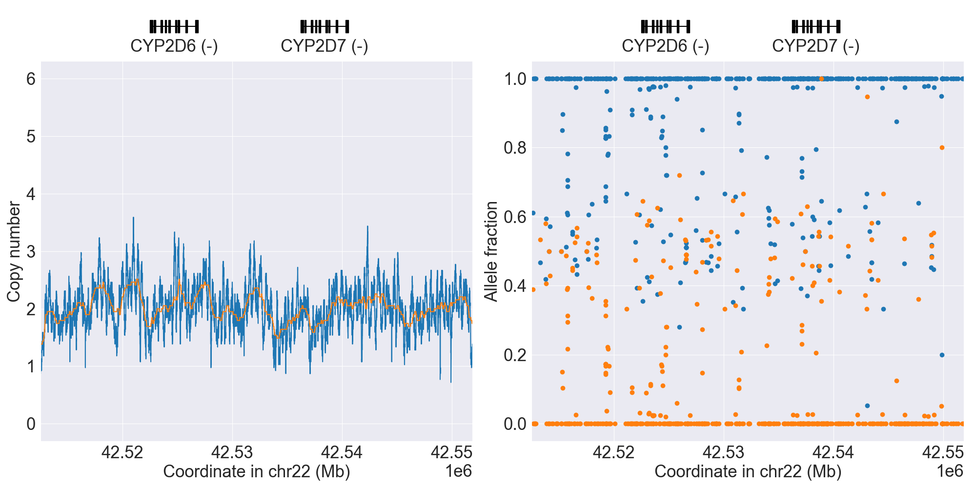
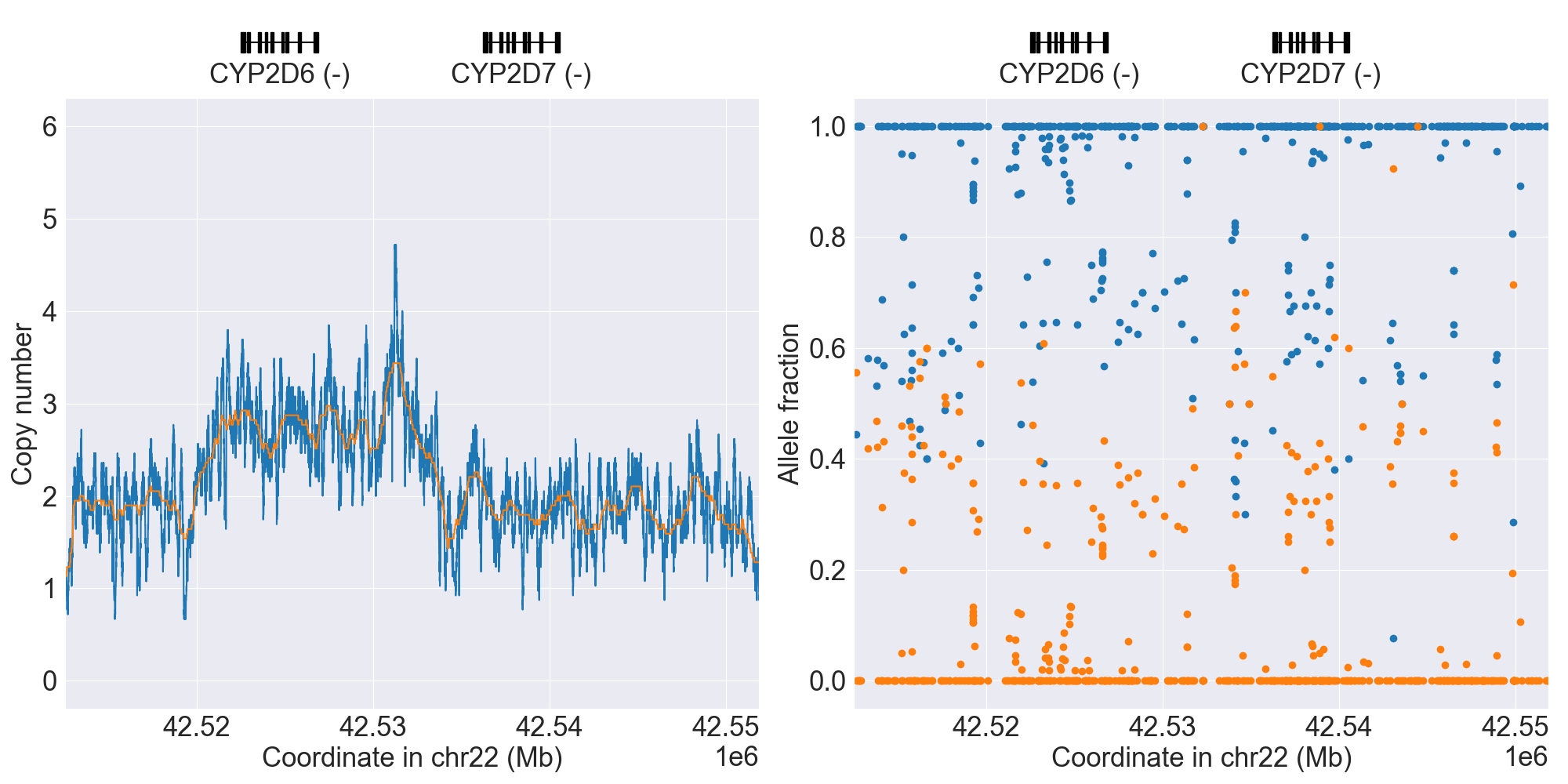
Next, we can manually inspect SV calls by visualizing copy number and allele
fraction for the CYP2D6 locus (read Structural variation detection for details). For example, above results indicate that the samples
HG00589_PyPGx and HG00436_PyPGx have Normal and WholeDup1
as CNV calls, respectively:
Sample |
Copy Number |
Allele Fraction |
|---|---|---|
HG00589_PyPGx |
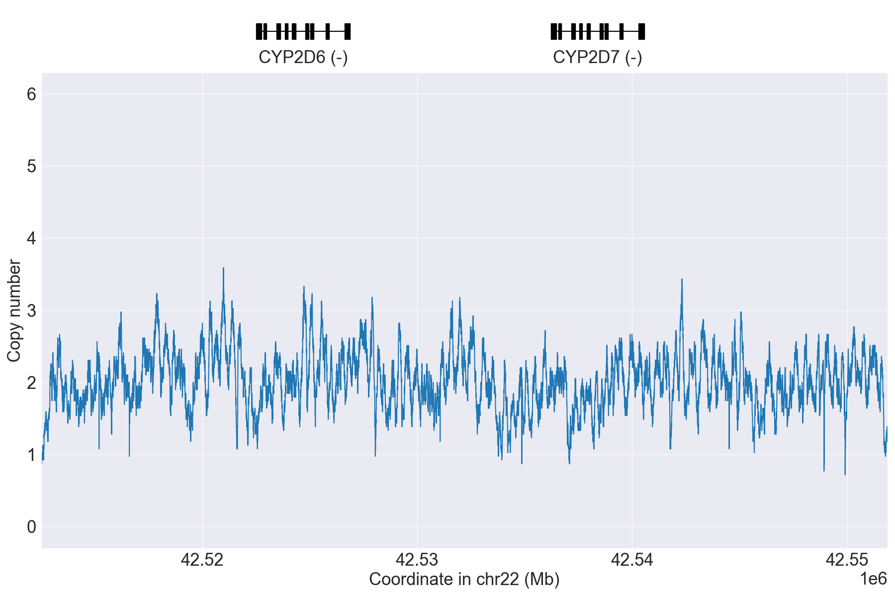
|
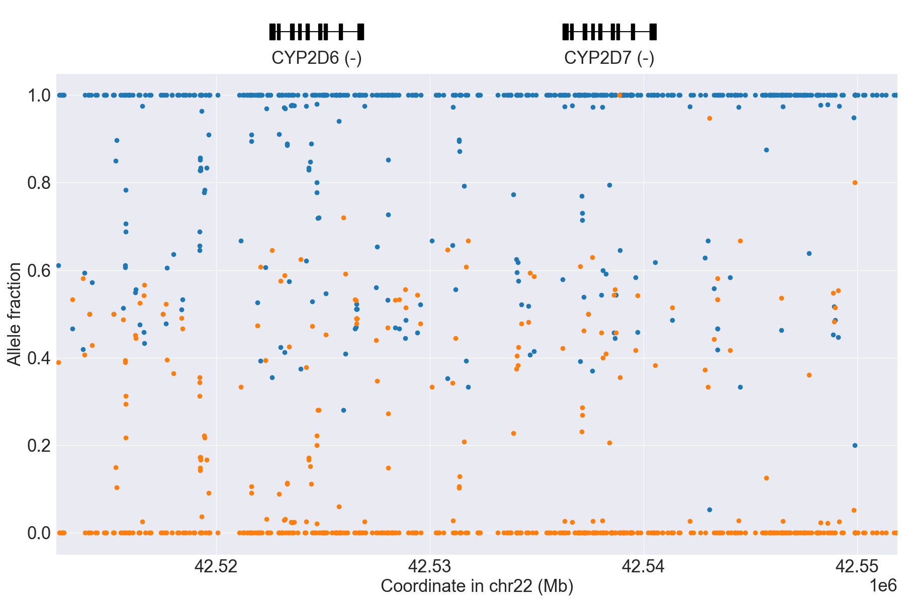
|
HG00436_PyPGx |
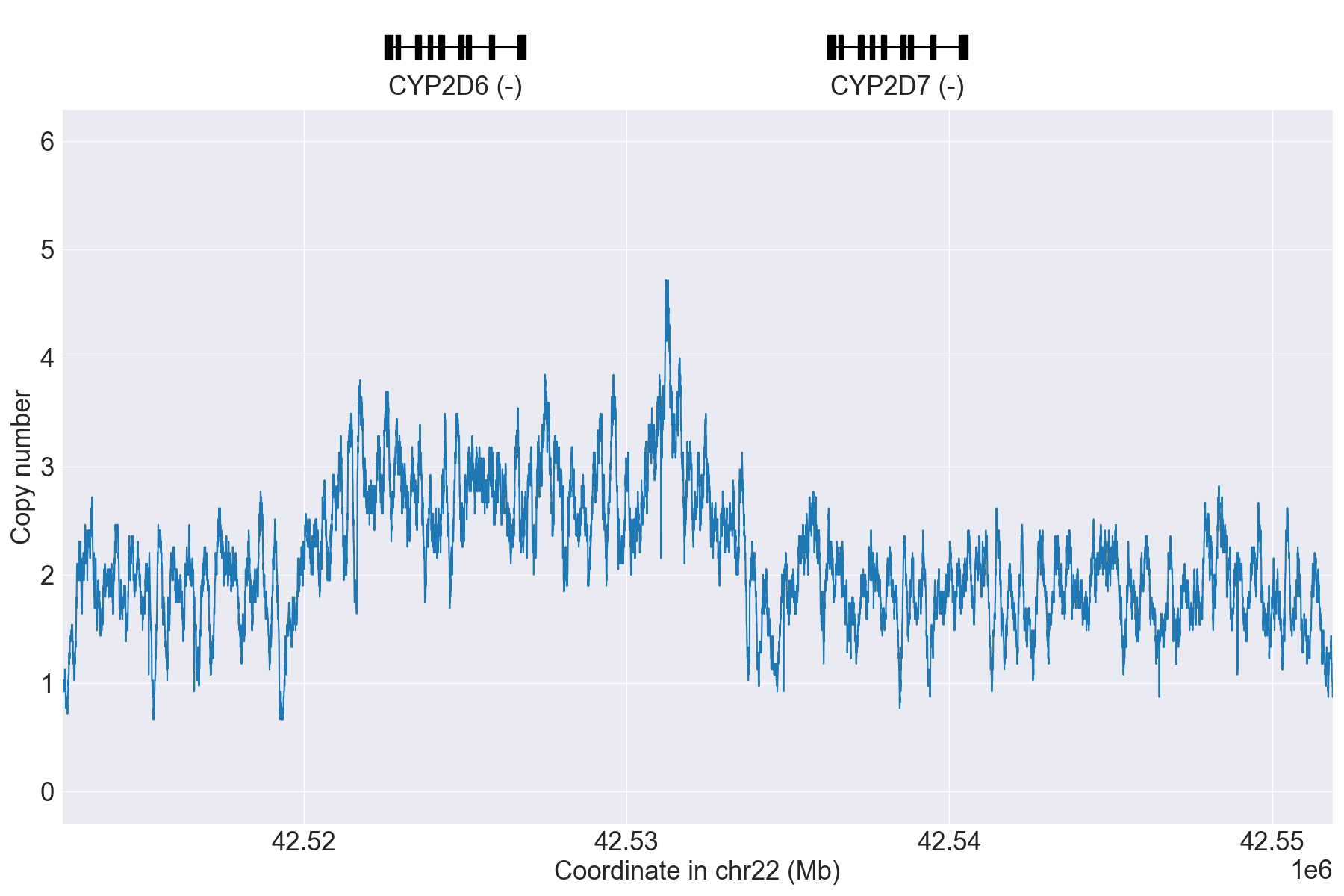
|
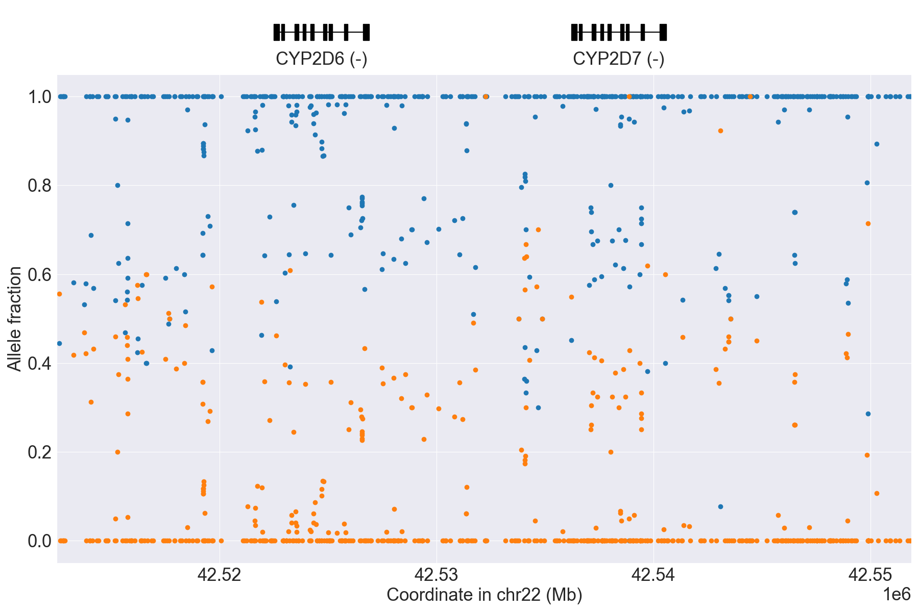
|
If you want to prepare publication quality figures, it’s strongly recommended to combine copy number and allele fraction profiles together:
$ pypgx plot-cn-af \
grch37-CYP2D6-pipeline/copy-number.zip \
grch37-CYP2D6-pipeline/imported-variants.zip \
--samples HG00589_PyPGx HG00436_PyPGx
Sample |
Profile |
|---|---|
HG00589_PyPGx |
|
HG00436_PyPGx |
|
Note that above also adds a fitted line on top of each copy number profile to display what the SV classifier actually “sees”.
Now let’s make sure the genotype results are correct by comparing them with the validation data:
$ wget https://raw.githubusercontent.com/sbslee/pypgx-data/main/getrm-wgs-tutorial/grch37-CYP2D6-results.zip
$ pypgx compare-genotypes grch37-CYP2D6-pipeline/results.zip grch37-CYP2D6-results.zip
# Genotype
Total: 70
Compared: 70
Concordance: 1.000 (70/70)
# CNV
Total: 70
Compared: 70
Concordance: 1.000 (70/70)
That’s it, you have successfully genotyped CYP2D6 with WGS data!
Genotyping genes without SV
The next gene we’re going to genotype is CYP3A5. Unlike CYP2D6, this gene
does not have any star alleles with SV. Therefore, we only need to provide
grch37-variants.vcf.gz to the NGS pipeline:
$ pypgx run-ngs-pipeline \
CYP3A5 \
grch37-CYP3A5-pipeline \
--variants grch37-variants.vcf.gz
Above will create a number of archive files:
Saved VcfFrame[Imported] to: grch37-CYP3A5-pipeline/imported-variants.zip
Saved VcfFrame[Phased] to: grch37-CYP3A5-pipeline/phased-variants.zip
Saved VcfFrame[Consolidated] to: grch37-CYP3A5-pipeline/consolidated-variants.zip
Saved SampleTable[Alleles] to: grch37-CYP3A5-pipeline/alleles.zip
Saved SampleTable[Genotypes] to: grch37-CYP3A5-pipeline/genotypes.zip
Saved SampleTable[Phenotypes] to: grch37-CYP3A5-pipeline/phenotypes.zip
Saved SampleTable[Results] to: grch37-CYP3A5-pipeline/results.zip
Plus the allele-fraction-profile directory.
Now you have successfully genotyped CYP3A5 as well!
Note
Note that if you provide grch37-depth-of-coverage.zip and
grch37-control-statistics-VDR.zip to the pipeline, PyPGx will still
run without any issues, but it will output a warning that says those
files will be ignored. This is so that users don’t have to memorize which
gene requires SV analysis. In other words, users can provide the same
input files for all target genes.
Genotyping with CRAM files
PyPGx also supports CRAM files as input.
$ mkdir grch37-cram
$ wget -P grch37-cram https://storage.googleapis.com/sbslee-bucket/pypgx/getrm-wgs-tutorial/grch37-cram/HG00276_PyPGx.sorted.markdup.recal.cram.crai
$ wget -P grch37-cram https://storage.googleapis.com/sbslee-bucket/pypgx/getrm-wgs-tutorial/grch37-cram/HG00276_PyPGx.sorted.markdup.recal.cram
$ wget -P grch37-cram https://storage.googleapis.com/sbslee-bucket/pypgx/getrm-wgs-tutorial/grch37-cram/HG00436_PyPGx.sorted.markdup.recal.cram.crai
$ wget -P grch37-cram https://storage.googleapis.com/sbslee-bucket/pypgx/getrm-wgs-tutorial/grch37-cram/HG00436_PyPGx.sorted.markdup.recal.cram
Similar to before, we will need the reference FASTA file used to create the CRAM files:
$ wget https://storage.googleapis.com/sbslee-bucket/ref/grch37/genome.fa
$ wget https://storage.googleapis.com/sbslee-bucket/ref/grch37/genome.fa.fai
We can create input files as usual:
$ pypgx create-input-vcf \
cram-variants.vcf.gz \
genome.fa \
grch37-cram/*.cram
$ pypgx prepare-depth-of-coverage \
cram-depth-of-coverage.zip \
grch37-cram/*.cram
$ pypgx compute-control-statistics \
VDR \
cram-control-statistics-VDR.zip \
grch37-cram/*.cram
Finally, we can run the NGS pipeline:
$ pypgx run-ngs-pipeline \
CYP2D6 \
cram-CYP2D6-pipeline \
--variants cram-variants.vcf.gz \
--depth-of-coverage cram-depth-of-coverage.zip \
--control-statistics cram-control-statistics-VDR.zip
$ pypgx print-data cram-CYP2D6/results.zip
    Genotype        Phenotype       Haplotype1      Haplotype2      AlternativePhase        VariantData     CNV
HG00276_PyPGx       *4/*5   Poor Metabolizer        *4;*10;*74;*2;  *4;*10;*74;*2;  ;       *4:22-42524947-C-T:0.87;*10:22-42523943-A-G,22-42526694-G-A:1.0,1.0;*74:22-42525821-G-T:1.0;*2:default; WholeDel1
HG00436_PyPGx       *2x2/*71        Indeterminate   *71;*1; *2;     ;       *71:22-42526669-C-T:0.433;*1:22-42523943-A-G,22-42522613-G-C:0.353,0.462;*2:default;    WholeDup1
Genotyping with GRCh38 data
Thus far, we have only considered GRCh37 data. But we can also run the
pipeline for GRCh38 data by changing the --assembly option:
$ pypgx run-ngs-pipeline \
CYP3A5 \
grch38-CYP3A5-pipeline \
--variants grch38-variants.vcf.gz \
--assembly GRCh38
Which will create:
Saved VcfFrame[Imported] to: grch38-CYP3A5-pipeline/imported-variants.zip
Saved VcfFrame[Phased] to: grch38-CYP3A5-pipeline/phased-variants.zip
Saved VcfFrame[Consolidated] to: grch38-CYP3A5-pipeline/consolidated-variants.zip
Saved SampleTable[Alleles] to: grch38-CYP3A5-pipeline/alleles.zip
Saved SampleTable[Genotypes] to: grch38-CYP3A5-pipeline/genotypes.zip
Saved SampleTable[Phenotypes] to: grch38-CYP3A5-pipeline/phenotypes.zip
Saved SampleTable[Results] to: grch38-CYP3A5-pipeline/results.zip
Now let’s make sure the genotype results are correct by comparing them with the GRCh37 results:
$ pypgx compare-genotypes grch37-CYP3A5-pipeline/results.zip grch38-CYP3A5-pipeline/results.zip
# Genotype
Total: 70
Compared: 70
Concordance: 1.000 (70/70)
# CNV
Total: 70
Compared: 0
Concordance: N/A
Congratulations, you have completed this tutorial!
Coriell Affy tutorial
In this tutorial I will show you how to genotype the CYP3A5 gene with chip data.
Coriell Institute has carried out Affy 6.0 genotyping on many of the 1000 Genomes Project (1KGP) samples whose data are available on 1KGP’s FTP site. For this tutorial we will be using the file ALL.wgs.nhgri_coriell_affy_6.20140825.genotypes_no_ped.vcf.gz which contains variant data for 355 samples.
For convenience, I prepared input files:
$ mkdir coriell-affy-tutorial
$ cd coriell-affy-tutorial
$ wget https://raw.githubusercontent.com/sbslee/pypgx-data/main/coriell-affy-tutorial/variants.vcf.gz
$ wget https://raw.githubusercontent.com/sbslee/pypgx-data/main/coriell-affy-tutorial/variants.vcf.gz.tbi
Next, run the chip pipeline:
$ pypgx run-chip-pipeline \
CYP3A5 \
CYP3A5-pipeline \
variants.vcf.gz
Above will create a number of archive files:
Saved VcfFrame[Imported] to: CYP3A5-pipeline/imported-variants.zip
Saved VcfFrame[Phased] to: CYP3A5-pipeline/phased-variants.zip
Saved VcfFrame[Consolidated] to: CYP3A5-pipeline/consolidated-variants.zip
Saved SampleTable[Alleles] to: CYP3A5-pipeline/alleles.zip
Saved SampleTable[Genotypes] to: CYP3A5-pipeline/genotypes.zip
Saved SampleTable[Phenotypes] to: CYP3A5-pipeline/phenotypes.zip
Saved SampleTable[Results] to: CYP3A5-pipeline/results.zip
Now that’s it! You have successfully genotyped CYP3A5 with chip data.